Empirical Analyses with EcoCoMix - Single Function
Source:vignettes/Empirical_single.Rmd
Empirical_single.RmdSetup
This is an R Markdown document describing how to use EcoCoMix to conduct BEF regression, or any community-level analyses. You will need to install and load multiple packages and data.
library(phytools)
library(tidyverse)
library(EcoCoMix)
data("KSR")
data("KSR_MLtree")
data("KSR_EF")
Let’s get the variane covariance matrix at species and community level.
VCV_sp <- vcv(KSR_MLtree) #species level phyologenetic covariance matrix using default (Brownian) model
VCV_sp <- VCV_sp[order(rownames(VCV_sp)),order(colnames(VCV_sp))]
VCV_comm <- get_comm_pair_r(KSR,VCV_sp)
The KSR_EF data have multiple ecosystem function.
head(KSR_EF)
#>   Plot Real.rich litter2012 ave.biomass  LAI mean.N.change poll_total flwr_total Mass.loss.2month Damage_effect bugs bug.rich
#> 1   X2         1      79.05    32.97333 1.67       -0.0015         20 43113.5000            3.362     0.0000000    9        7
#> 2   X3         4      74.23    82.41000 5.53       -0.0275         53  2126.1429            3.718     0.3001195    7        6
#> 3   X4         2      34.50    62.92667 3.04        0.0060        150   324.4286            3.521     0.4195279    4        2
#> 4   X7         1      36.32    34.38333 3.42       -0.0575          0     0.0000            3.328     0.0000000    5        3
#> 5   X8         3      21.46   147.05667 7.14       -0.0070          0     0.0000            3.608     2.7460093    4        4
#> 6   X9         1      37.26    33.80333 1.01        0.0415          0     0.0000            3.627     0.0000000   11        7
Data Description
| Variable | Description |
|---|---|
| Plot | Plot identity |
| Real.rich | Number of species planted |
| litter2012 | Amount of litter measured in 2012 |
| ave.biomass | Average biomass across 2012-2014 |
| LAI | Leaf area index, a simplified dimension of structural complexity |
| mean.N.change | delta 15N change averaged across surface and deep soil |
| poll_total | Total number of pollinators |
| flwr_total | Total number of flowers |
| Mass.loss.2month | Decomposition after 2 months |
| Damage_effect | Damage reduction effect |
| bugs | Total number of arthropods |
| bug.rich | Species richness of arthropods |
Empirical Analyses - Single Function
Here we reanalyze the data in Cadotte et al. (2017), involving ten ecosystem functions.
Let’s say we are only interested in LAI. For compositional random effect, please designate the random effect as corrMatrix(1|comp_id) in EcoCoMix (even though you might not have the column comp_id in the data frame.). The function will automatically generate a column comp_id in the internal calculation (i.e., every community will have an unique identifier).
m_LAI <- EcoCoMix(LAI~Real.rich+corrMatrix(1|comp_id),
                                     data=KSR_EF,
                                     comm=KSR,
                                     VCV_sp = vcv(KSR_MLtree),
                                     method.spaMM="REML",
                                     init=list())

summary(m_LAI$best_model)
#> formula: LAI ~ Real.rich + corrMatrix(1 | comp_id)
#> Estimation of fixed effects by ML.
#> Estimation of lambda and phi by 'outer' REML, maximizing restricted logL.
#> family: gaussian( link = identity )
#>  ------------ Fixed effects (beta) ------------
#>             Estimate Cond. SE t-value
#> (Intercept)   2.6197   0.5147   5.089
#> Real.rich     0.7042   0.2482   2.838
#>  --------------- Random effects ---------------
#> Family: gaussian( link = identity )
#>            --- Variance parameters ('lambda'):
#> lambda = var(u) for u ~ Gaussian;
#>    comp_id  :  5.407
#> # of obs: 88; # of groups: comp_id, 88
#>  -------------- Residual variance  ------------
#> phi estimate was 1.68569
#>  ------------- Likelihood values  -------------
#>                         logLik
#> logL       (p_v(h)): -167.5682
#> Re.logL  (p_b,v(h)): -167.9030
m_LAI$best_model_satt #Satterthwaite's method is better for p-values.
#> Single term deletions using Satterthwaite's method:
#>
#> Model:
#> LAI ~ Real.rich + corrMatrix(1 | comp_id)
#>           Sum Sq Mean Sq NumDF  DenDF F value Pr(>F)
#> Real.rich 13.573  13.573     1 14.232   8.052  0.013 *
#> ---
#> Signif. codes:  0 '***' 0.001 '**' 0.01 '*' 0.05 '.' 0.1 ' ' 1
get_R2(m_LAI$best_model) #get R2 too
#>        R2m        R2c
#> 0.07936676 0.78118520
Note that EcoCoMix also returns outputs of other models (not just the best model). For example, if you are interested in the model based on the provided correlation matrix
m_LAI$original_VCV_model
#> formula: LAI ~ Real.rich + corrMatrix(1 | comp_id)
#> Estimation of fixed effects by ML.
#> Estimation of lambda and phi by 'outer' REML, maximizing restricted logL.
#> family: gaussian( link = identity )
#>  ------------ Fixed effects (beta) ------------
#>             Estimate Cond. SE t-value
#> (Intercept)   3.5942   1.2294   2.924
#> Real.rich     0.9348   0.2287   4.087
#>  --------------- Random effects ---------------
#> Family: gaussian( link = identity )
#>            --- Variance parameters ('lambda'):
#> lambda = var(u) for u ~ Gaussian;
#>    comp_id  :  67.24
#> # of obs: 88; # of groups: comp_id, 88
#>  -------------- Residual variance  ------------
#> phi estimate was 1.73291
#>  ------------- Likelihood values  -------------
#>                         logLik
#> logL       (p_v(h)): -175.7253
#> Re.logL  (p_b,v(h)): -175.4702
m_LAI$original_VCV_m_satt
#> Single term deletions using Satterthwaite's method:
#>
#> Model:
#> LAI ~ Real.rich + corrMatrix(1 | comp_id)
#>           Sum Sq Mean Sq NumDF  DenDF F value    Pr(>F)
#> Real.rich  28.95   28.95     1 68.943  16.706 0.0001162 ***
#> ---
#> Signif. codes:  0 '***' 0.001 '**' 0.01 '*' 0.05 '.' 0.1 ' ' 1
get_R2(m_LAI$original_VCV_model)
#>        R2m        R2c
#> 0.01538212 0.97526177
Details about all results provided by EcoCoMix are provided here.
Residual Checking
Let’s do some model diagnostics to make sure our model makes sense. The package DHARMa supports output from spaMM, so we will use it for model diagnostics.
library(DHARMa)
#> Warning: package 'DHARMa' was built under R version 4.3.3
#> This is DHARMa 0.4.7. For overview type '?DHARMa'. For recent changes, type news(package = 'DHARMa')

sres <- simulateResiduals(m_LAI$best_model)
plot(sres)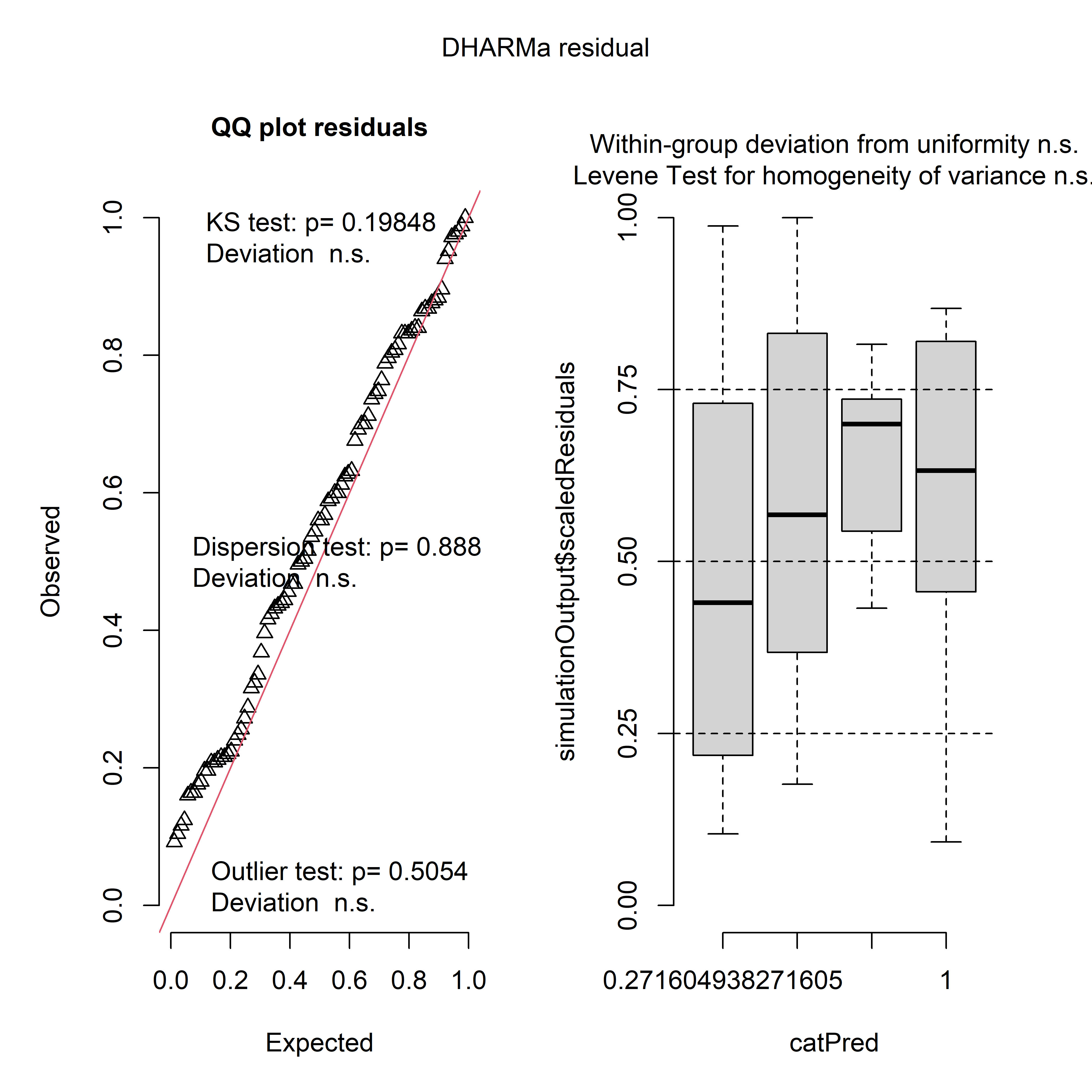
Outputs from DHARMa for the negative binomial model
Making figures
Let’s say we want to visualize the predicted relationships between LAI and species richness. In spaMM, you can use the predict function to obtain model predictions with/without random effects. In our case, we just need to generate a new dataset that include the species richness gradient, and provide it to the predict function.
library(ggplot2)

newdata <- data.frame(Real.rich=unique(KSR_EF$Real.rich)) #create a new data frame for the predictions

predict_df <- predict(m_LAI$best_model,newdata=newdata,re.form=NA,variances=list(fixefVar=TRUE),intervals="fixefVar",binding="Response") #prediction based on fixed effect only

predict_df <- cbind(predict_df,attr(predict_df,"intervals")) #restructuring the data such that the mean predictions and their 2.5 and 97.5% CI are in the same data frame.

p <- ggplot()+
  geom_point(data=KSR_EF,aes(x=Real.rich,y=LAI))+
  geom_line(data=predict_df,aes(x=Real.rich,y=Response))+
  geom_ribbon(data=predict_df,aes(x=Real.rich,y=Response,ymin=fixefVar_0.025,ymax=fixefVar_0.975),alpha=0.3)+
  labs(x="Species richness",y = "LAI")+
  theme_classic()

plot(p)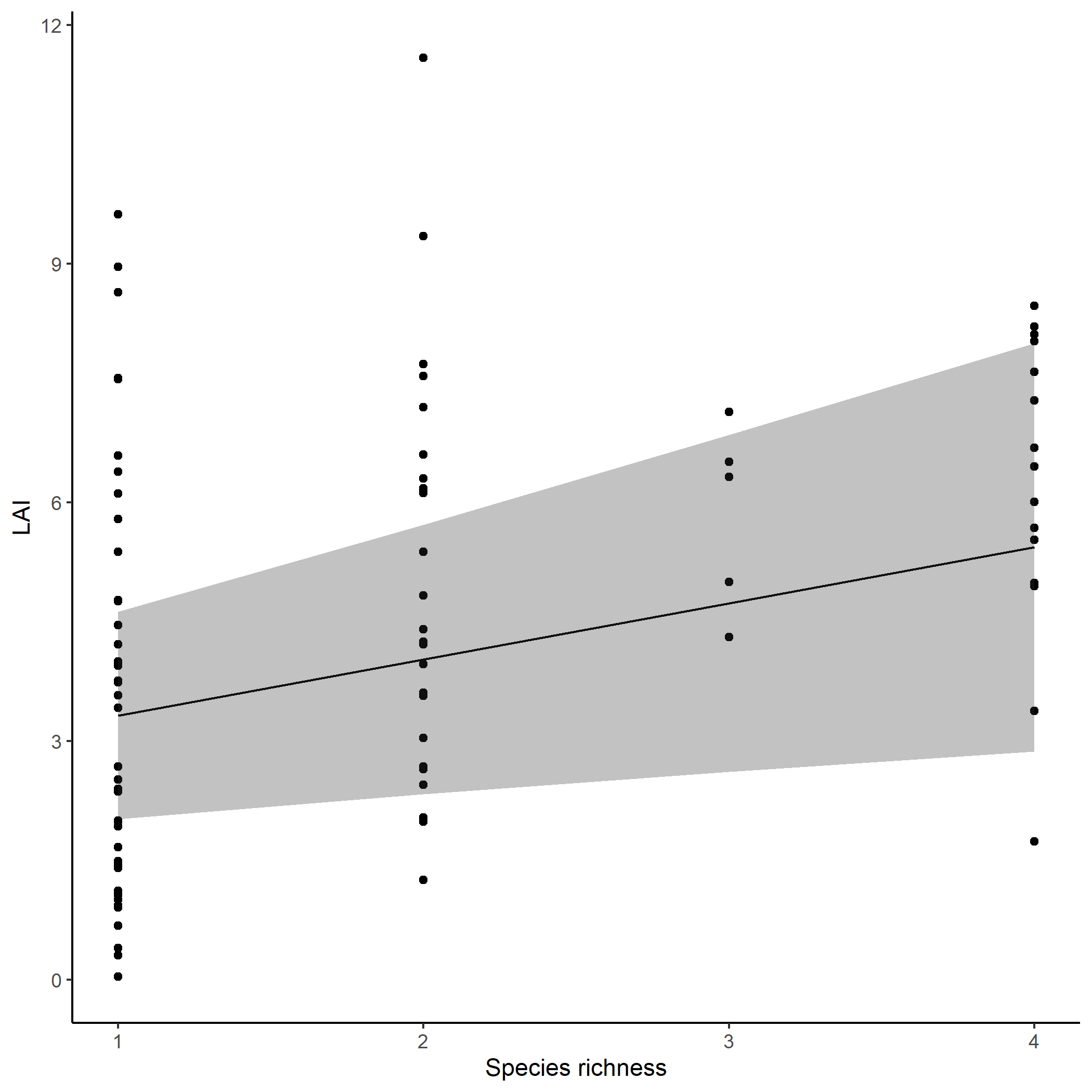
Predicted effects of species richness on LAI